Basket Analysis in Power BI

Aaa, give me some Sales data…

Some business requirements sometimes … “require” more than an analytical tool of choice can allow us to create.

Let me explain.

In the past something like this was the area of Data Mining.

(Data Mining is an somewhat retired expression, nowadays this is called more like Data Science.)

In the old days analyses that were a little to complex for SQL or simple OLAP cube were put aside for the expensive in-depth Data Mining tools.

Let’s for instance take the Shopping Basket Analysis as an example.

You ask an engineer and he will tell you that this is quadratic or even a n! (factorial) problem … going on an on …

Write SQL code that computes the result … that’s a lot of code!

But thanks to the guys at SQLBI it is not as hard.

Let us look at an example data model of a Sales fact table and some dimension tables (star schema).

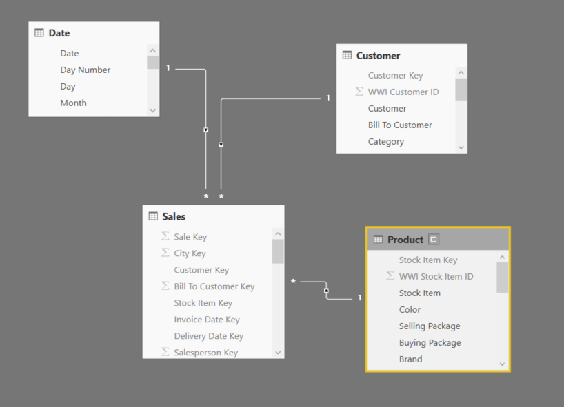
Starting with such example, we are given a Fact table with the Product dimension linked to it.

And actually this is all we need.

We want to be able to compare sales of a product or item with another product or item.

And thanks to the DAX engine we are able to just do that.

In a calculation. Based on a user’s selection.

Before going to write the calculation, what we need is a second Product table that will be used for the other product in the comparison.

This is easy to do in Power BI.

We just materialize in-memory a second identical table in the data model.

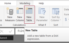
Modelling tab => New Table

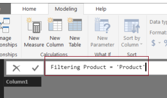
Writing the name of the new table equals (=) the name of the existing one – Prodcut

Connect the additional Product table to the fact Sales with a non-active relationship to not bother the model in a direct way.

And the calculation is about this one:
Both Products Bought =
CALCULATE (
    DISTINCTCOUNT ( Sales[Sale Key] );
    CALCULATETABLE (
        SUMMARIZE ( Sales; Sales[Sale Key] );
        ALL ( Product );
        USERELATIONSHIP ( Sales[Stock Item Key]; ‘Filter Product'[Stock Item Key] )
    )
)

What do we do there…

Some DAX code familiarity will help…

Nonetheless:

1. Take Sales Orders – SUMMARIZE function
2. Remove filters on Product table (ALL function) – as where the first product is selected
3. To calculate use the inactive relationship that we have previously created (USERELATIONSHIP)
4. Count, distinctly (as many lines of the same product can be on one order) of the number of orders that are filtered by “normal” filters – mainly the original Product table, but as well as Date filter, etc. …. AND by filtering only those orders that we precomputed in the 1-3 steps.

Together the calculation gives us the number of orders that one product from the Product table is selected and also where a second product from table Filtering Product is selected.

With a little tweaking we can get useful use cases:

1. Which items were mostly bought with selected item

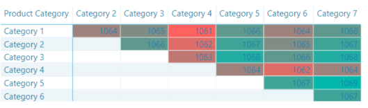
2. Item Correlation heatmap

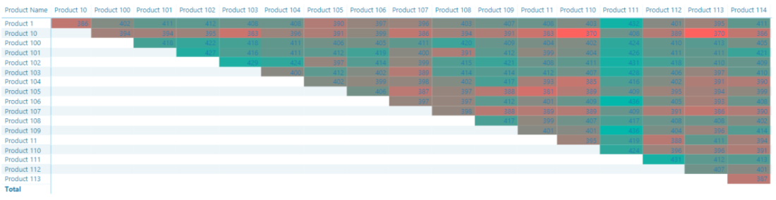
3. Item category / Product Group heatmap

Power BI has come a long way from where it started (only as a Excel add-on). It has a very versatile and powerful in-memory calculation engine called the DAX engine (or xVelocity more technically). I have been using Power BI to gain insights from its inception, year 2015.